User Guide
Installation
you can install ooipy with pip
pip install ooipy
If you want to get latest (unreleast) versions, or contribute to development you can clone the repository and install it from the source code.
git clone https://github.com/Ocean-Data-Lab/ooipy.git
cd ooipy
pip install -e .
The -e flag allows you to edit the source code and not have to reinstall the package.
The installation has several extras for different development cases [‘dev’,’docs’]. These optional dependencies can be installed with pip install -e .[dev] or pip install -e .[docs].
Download Hydrophone Data
How to download data from broadband hydrophones
import ooipy
import datetime
from matplotlib import pyplot as plt

# Specify start time, end time, and node for data download (1 minutes of data)
start_time = datetime.datetime(2017,7,1,0,0,0)
end_time = datetime.datetime(2017,7,1,0,1,0)
node1 = 'LJ01D'

# Download Broadband data
print('Downloading Broadband Data:')
hdata_broadband = ooipy.get_acoustic_data(start_time, end_time, node1, verbose=True)
How to download data from low frequency hydrophones
start_time = datetime.datetime(2017,7,1,0,0,0)
end_time = datetime.datetime(2017,7,1,0,1,0)
node='Eastern_Caldera'

# Download low frequency data
print('Downloading Low Frequency Data:')
hdata_lowfreq = ooipy.get_acoustic_data_LF(start_time, end_time, node2, verbose=True, zero_mean=True)
The ooipy.hydrophone.basic.HydrophoneData() object has all of the functionality of the obspy.core.trace.Trace, which includes plotting, resampling, filtering and more. See obspy documentation for more information.
Hydrophone nodes
Broadband Hydrophones
Oregon Shelf Base Seafloor (Fs = 64 kHz)
‘LJ01D’
Oregon Slope Base Seafloor (Fs = 64 kHz)
‘LJ01A’
Slope Base Shallow (Fs = 64 kHz)
‘PC01A’
Axial Base Shallow Profiler (Fs = 64 kHz)
‘PC03A’
Offshore Base Seafloor (Fs = 64 kHz)
‘LJ01C’
Axial Base Seafloor (Fs = 64 kHz)
‘LJ03A’
Low Frequency Hydrophones
Axial Base Seaflor (Fs = 200 Hz)
‘Axial_Base’
‘AXABA1’
-
‘Central_Caldera’
‘AXCC1’
-
‘Eastern_Caldera’
‘AXEC2’
Southern Hydrate (Fs = 200 Hz)
‘Southern_Hydrate’
‘HYS14’
‘Oregon Slope Base Seafloor (Fs = 200 Hz)
‘Slope_Base’
‘HYSB1’
For more detailed information about hydrophones nodes see https://ooinet.oceanobservatories.org/
Here is a map of hydrophones supported by OOIpy
Compute PSDs and Spectrograms
The ooipy.hydrophone.basic.HydrophoneData data object, which is a wrapper for the obspy.core.trace.Trace provides methods to compute Power Spectral Densities, and Spectrograms. The spectrograms are actually multiple power-spectral density estimates as a function of time, instead of a typical short-time fourier transform, such as scipy.signal.stft().
The OOI hydrophones often have colocated instruments that can corrupt than ambient sound measurements. We’ve found that the welch method with median averaging [1] gives the best result for power spectral density estimates, and is what has been used for much research on spectral levels with OOI hydrophones [2][3][4]
Calibration
ooipy also handles calibration of the hydrophones. The low-frequency hydrophones were calibrated before their deployment in 2014, and have not been calibrated since. The calibration information for the low frequency hydrophones can be found on the IRIS website.
The broadband hydrophones are recovered every year and calibrated by Ocean Sonics, the information about hydrophone deployments can be found here, and the calibration sheets can be found here.
Warning
Calibration needs to be updated. The deployments and calibration files are not updated past 2021.
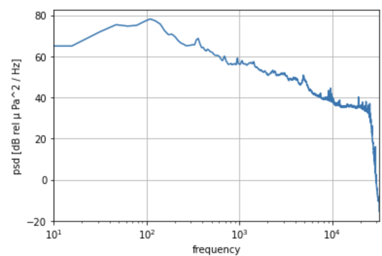
compute Power spectral density
Use the ooipy.hydrophone.basic.HydrophoneData.compute_psd_welch() method to estimate the power spectral density. The power spectral density estimate is returned as an xarray.DataArray.
psd1 = hdata_broadband.compute_psd_welch()
psd1.plot()
plt.xlim([10,32000])
plt.grid()
plt.xscale('log')
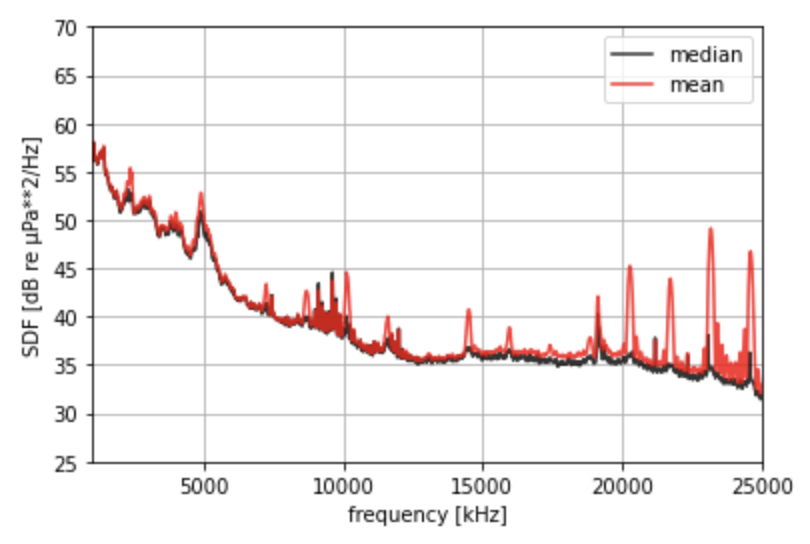
difference between different averaging methods
# power spectral density estimate of noise data using Welch's method
fig, ax = plt.subplots(figsize=(6,4))

# 1. using median averaging (default)
psd_med = hdata_broadband.compute_psd_welch()

# 2. using mean averaging
psd_mean = hdata_broadband.compute_psd_welch(avg_method='mean')

psd_med.plot(c='k', alpha=0.8, label='median')
psd_mean.plot(c='r', alpha=0.8, label='mean')


plt.xlabel('frequency [kHz]')
plt.ylabel('SDF [dB re µPa**2/Hz]')
plt.xlim(1000,25000)
plt.ylim(25,70)
plt.legend()
plt.grid()
Compute Spectrogram
Use the ooipy.hydrophone.basic.HydropheData.compute_spectrogram() method to compute the spectrogram.
spec1 = hdata_broadband.compute_spectrogram()
Batch hydrophone downloads
There is a program for batch downloading ooi hydrophone data provided with the installation of ooipy. You can access it from your terminal:
download_hydrophone_data --csv <path to csv> --output_path <path to save files>
Here is an example csv file:
node,start_time,end_time,file_format,downsample_factor
LJ03A,2019-08-03T08:00:00,2019-08-03T08:01:00,wav,1
AXBA1,2019-08-03T12:01:00,2019-08-03T12:02:00,wav,1
Download CTD Data
Warning
CTD downloads currently works, but are not actively supported. You should first look at the OOI Data Explorer.
import packages and initialize your api token
import ooipy
import datetime
from matplotlib import pyplot as plt

USERNAME = <'YOUR_USERNAME'>
TOKEN =  <'YOUR_TOKEN'>
ooipy.request.authentification.set_authentification(USERNAME, TOKEN)
request 1-hour of CTD data from the oregonoffshore location
start = datetime.datetime(2016, 12, 12, 2, 0, 0)
end = datetime.datetime(2016, 12, 12, 3, 0, 0)
ctd_data = ooipy.request.ctd_request.get_ctd_data(start, end, 'oregon_offshore', limit=10000)
print('CTD data object: ', ctd_data)
print('number of data points: ', len(ctd_data.raw_data))
print('first data point: ', ctd_data.raw_data[0])
request 1-day of CTD data from the oregonoffshore location
import time
day = datetime.datetime(2016, 12, 12)
t = time.time()
ctd_data = ooipy.request.ctd_request.get_ctd_data_daily(day, 'oregon_offshore')
print(time.time() - t)
print('CTD data object: ', ctd_data)
print('number of data points: ', len(ctd_data.raw_data))
print('first data point: ', ctd_data.raw_data[0])
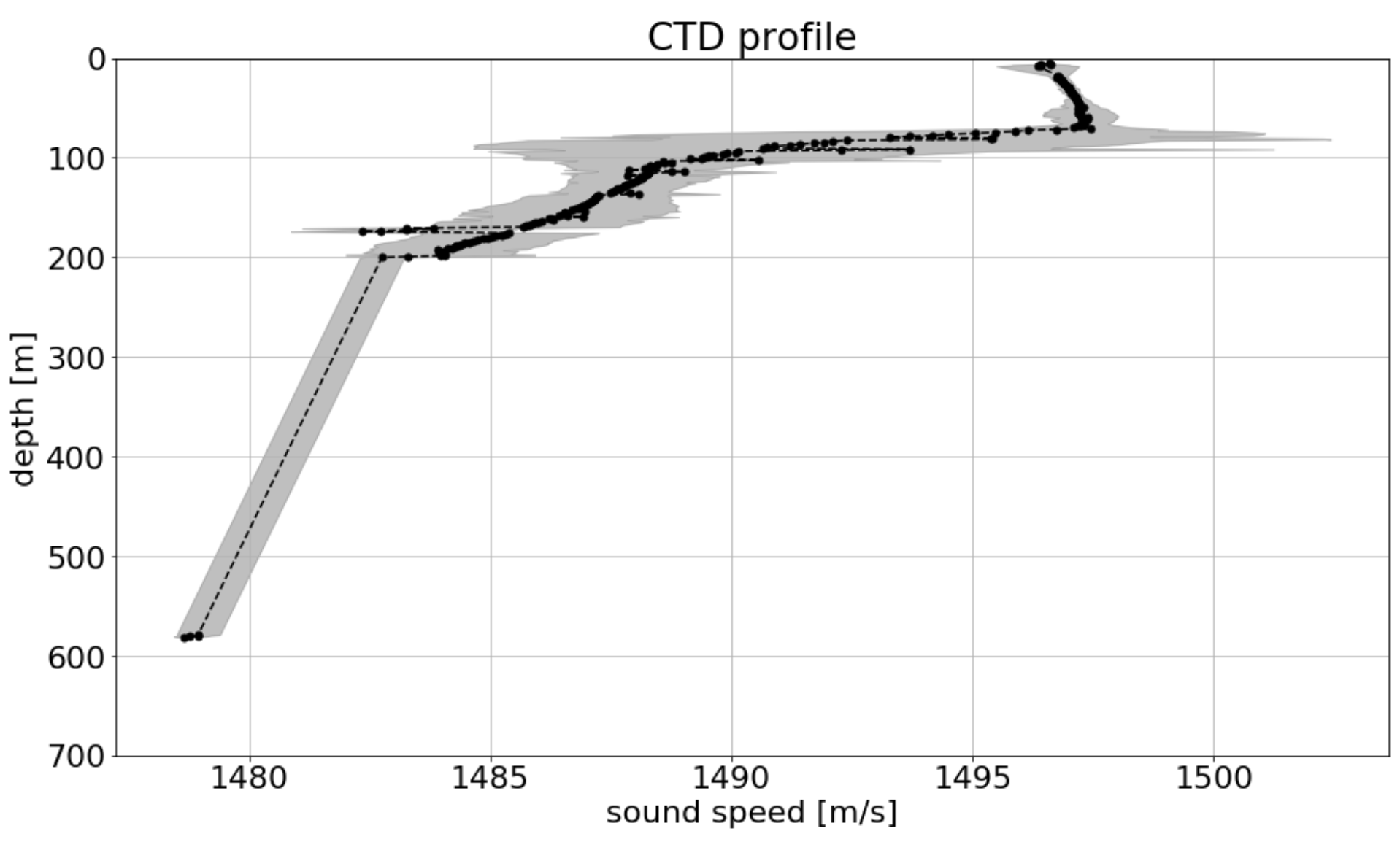
compute sound speed profile for daily data
c_profile = ctd_data.get_profile(600, 'sound_speed')
plot ctd profile mean and standard deviation
c_profile.plot(xlabel='sound speed')